1.1 Getting Data for Assessing Ecosystem Services

You have learned about different ecosystem assessment tools available in InVEST. We will now go in depth with water yield to assess the hydropower production from reservoirs service.

Hydropower accounts for 20% of worldwide energy production, most of which is generated by reservoir systems. InVEST estimates the annual average quantity and value of hydropower produced by reservoirs and identifies how much water yield or value each part of the landscape contributes annually to hydropower production.

The model has three components: water yield, water consumption, and hydropower valuation. The first two components use data on average annual precipitation, annual reference evapotranspiration and a correction factor for vegetation type, root restricting layer depth, plant available water content, land use and land cover, root depth, elevation, saturated hydraulic conductivity, and consumptive water use. The valuation model uses data on hydropower market value and production costs, the remaining lifetime of the reservoir, and a discount rate.

Upon completion of this exercise, participants should be able to:

• Install InVEST package and choose a specific ecosystem services model

• Identify the input data needed to run the InVEST model: Water Yield

• Define a specific location for a case study

• Find this data on the Internet and download it

1.1.1 Install InVEST and choose your model

First, we search for the InVEST model on the NatCap website at : http://www.naturalcapitalproject.org/invest

Once identified, you can download the latest version of the package without the tutorial data. The InVEST package is a standalone software that will run on Windows or Mac operating systems.

1.1.2 Identify the geospatial data inputs

As described in the InVEST User manual under the Water Yield model the data needed for this model (http://data.naturalcapitalproject.org/nightly-build/invest-users-guide/html) is presented below:

1. Precipitation (required). A geographic information System (GIS) raster dataset with a non-zero value for average annual precipitation for each cell. The precipitation values should be in millimeters.

2. Average Annual Reference Evapotranspiration (required). A GIS raster dataset, with an annual average evapotranspiration value for each cell. Reference evapotranspiration is the potential loss of water from soil by both evaporation from the soil and transpiration by healthy alfalfa (or grass) if sufficient water is available. The reference evapotranspiration values should be in millimeters.

3. Root restricting layer depth (required). A GIS raster dataset with an average root restricting layer depth value for each cell. Root restricting layer depth is the soil depth at which root penetration is strongly inhibited because of physical or chemical characteristics. The root restricting layer depth values should be in millimeters.

4. Plant Available Water Content (required). A GIS raster dataset with a plant available water content value for each cell. Plant Available Water Content fraction (PAWC) is the fraction of water that can be stored in the soil profile that is available for plants’ use. PAWC is a fraction from 0 to 1.

5. Land use/land cover (required). A GIS raster dataset, with an LULC code for each cell. The LULC code should be an integer.

6. Watersheds (required). A shapefile, with one polygon per watershed. This is a layer of watersheds such that each watershed contributes to a point of interest where hydropower production will be analyzed.

7. Subwatersheds (required). A shapefile, with one polygon per subwatershed within the main watersheds specified in the Watersheds shapefile.

The standard GIS raster file formats should be used (e.g., ESRI GRID, TIF or IMG) or vector formats (ESRI shapefiles). The necessary GIS files can be named anything, but no spaces in the name and less than 13 characters if an ESRI GRID. If a TIF or IMG, the name may be longer. We will learn how to pre-process this data in the next exercise (part 6.3). More details on the data needed for the Water Yield model can be found at:

http://data.naturalcapitalproject.org/nightly-build/invest-users-guide/html/reservoirhydropowerproduction.html#data-needs

Once you have downloaded the required files you will have to pre-process them in the open source QGIS software in the next exercise. Each dataset must be in the right format with the correct spatial extent and the same geographic projection.

1.1.3 Area of Interest

Choose a location where you would like to assess water yield with InVEST. We have chosen our hometown of Geneva in Switzerland.

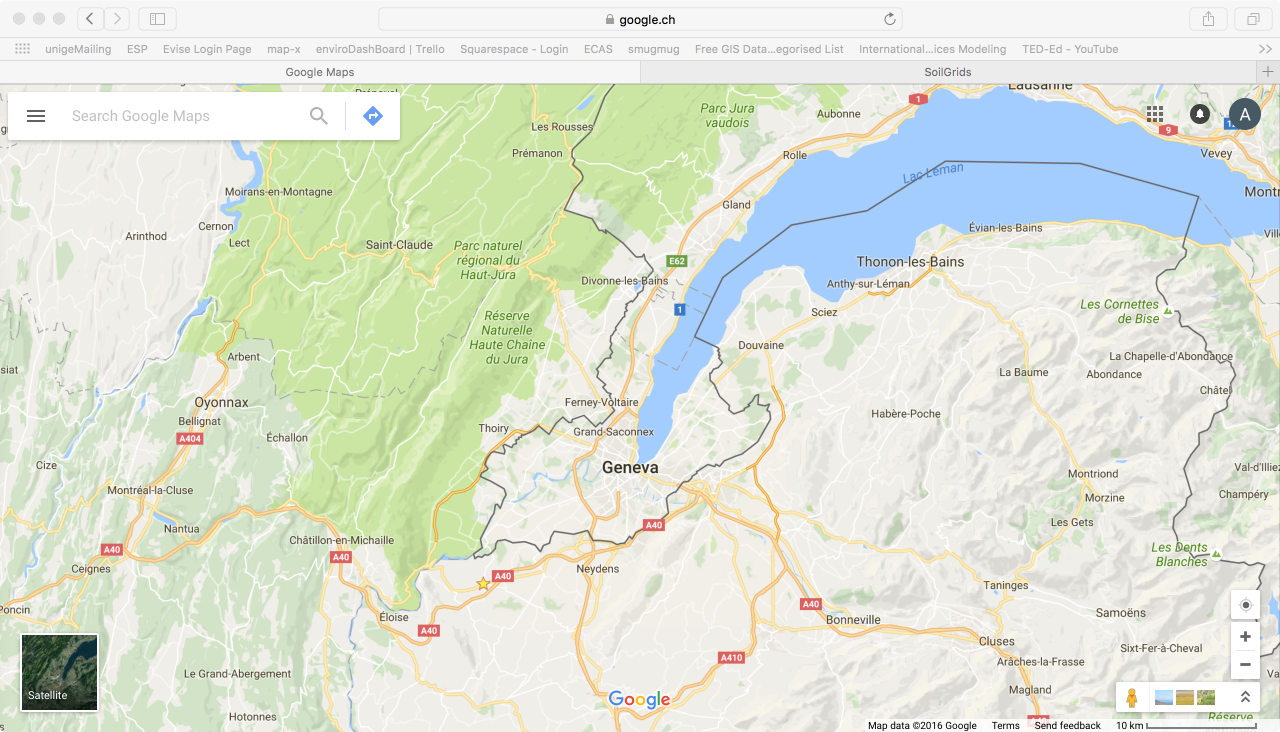
We first need to find the geographic coordinates for the extent of the area of interest (AOI). We suggest using Google Map for this with http://maps.google.com, and clicking on the lower left and upper right corners of your AOI, and then writing down the coordinates.

Figure 0.1: Google Map view of Geneva, Switzerland

In the case of Geneva it could be:

Lower left corner: 46.109818 N, 5.940873 E

Upper right corner: 46.444043 N, 6.421520 E

These coordinates will be useful to select our input data in the next steps and to clip the data to the useful extent if needed.

1.1.4 Precipitation

Global annual precipitation data can be obtained from the WorldClim dataset at 1km resolution: http://www.worldclim.org/ (Fick & Hijmans, 2017). For Geneva we selected the tile 16 and downloaded Precipitation in Geotiff format.

Figure 0.2: Map of WorldClim tile grid of global precipitation data

Alternatively select your tile from the following table:

XX	X0	X1	X2	X3	X4	X5	X6	X7	X8	X9	X10	X11
0X	00	01	02	03	04	05	06	07	08	09	010	011
1X	10	11	12	13	14	15	16	17	18	19	110	111
2X	20	21	22	23	24	25	26	27	28	29	210	211
3X	30	31	32	33	34	35	36	37	38	39	310	311
4X	40	41	42	43	44	45	46	47	48	49	410	411

Table 1: Table of WorldClim tile grid of global precipitation data

1.1.5 Average Annual Reference Evapotranspiration

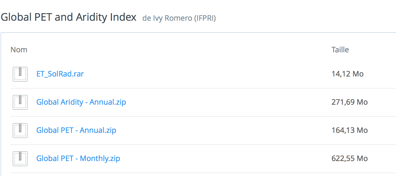
Global annual reference evapotranspiration may be obtained from the CGIAR CSI dataset (based on WorldClim data): http://www.cgiar-csi.org/data/global-aridity-and-pet-database (Zomer et al., 2007). The Annual Global-PET dataset is provided for non-commercial use in standard ARC/INFO Grid format, at 30 arc seconds (~ 1km at equator), to support studies contributing to sustainable development, biodiversity and environmental conservation, poverty alleviation, and adaption to climate change globally, and in particular in developing countries.

Figure 0.3: Screenshot of DropBox folder for global potential evapotranspiration and aridity index data

Figure 0.4: Map of global potential evapotranspiration data

1.1.6 Plant Available Water Content and Root Restricting Layer Depth

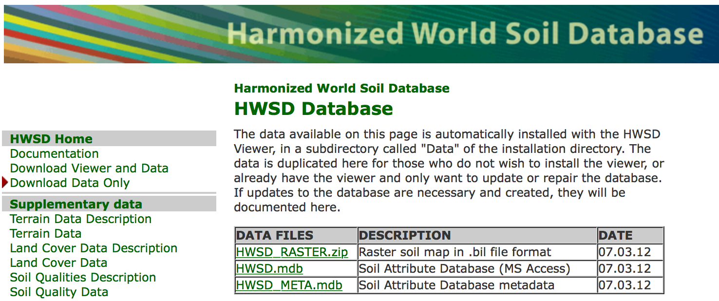
Depth to root restricting layer can be derived from The FAO global soil data in their Harmonized World Soil Database (HWSD): http://webarchive.iiasa.ac.at/Research/LUC/External-World-soil-database/HTML/HWSD_Data.html (FAO/IIASA/ISRIC/ISSCAS/JRC, 2012). The HWSD is a 30 arc-second raster database with over 16000 different soil mapping units that combines existing regional and national updates of soil information worldwide (SOTER, ESD, Soil Map of China, WISE) with the information contained within the 1:5’000’000 scale FAO-UNESCO Soil Map of the World.

Figure 0.5: Screenshot of Harmonized World Soil Database download page

1.1.7 Land Use Land Cover

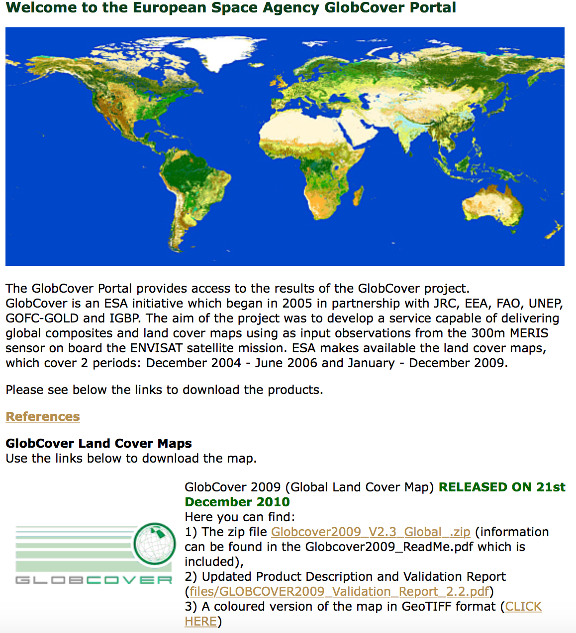
Land use: Global land use data for 2009 is available at 300m resolution from: the European Space Agency: http://due.esrin.esa.int/page_globcover.php (Arino et al., 2012). GlobCover is an ESA initiative that began in 2005 in partnership with JRC, EEA, FAO, UNEP, GOFC-GOLD and IGBP. The aim of the project was to develop a service capable of delivering global composites and land cover maps using as input observations from the 300m MERIS sensor on board the ENVISAT satellite mission.

Figure 0.6: Map of GlobCover global landuse and land cover data

Figure 0.7: Screenshot of GlobCover global landuse and land cover download page

1.1.8 Watersheds

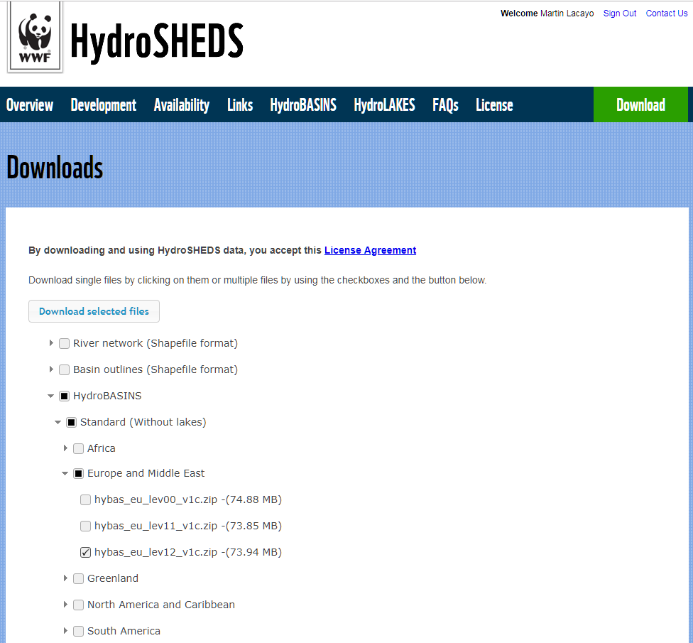
Watersheds and subwatersheds: http://hydrosheds.org/page/hydrobasins (Lehner & Grill, 2013). HydroBASINS is a series of polygon layers that depict watershed boundaries and sub-basin delineations at a global scale. The goal of this product is to provide a seamless global coverage of consistently sized and hierarchically nested sub-basins at different scales (from tens to millions of square kilometers), supported by a coding scheme that allows for analysis of watershed topology such as up- and downstream connectivity. The HydroBASINS product has been developed on behalf of World Wildlife Fund US (WWF), with support and in collaboration with the EU BioFresh project, Berlin, Germany; the International Union for Conservation of Nature (IUCN), Cambridge, UK; and McGill University, Montreal, Canada.

Figure 0.8: Screenshot of HydroSHEDS global watershed data

1.1.9 Biophysical Table

For data sources and estimation methods seehttp://data.naturalcapitalproject.org/nightly-build/invest-users-guide/html/reservoirhydropowerproduction.html#appendix-a-data-sources.

The following resources are suggested:

Schenk, H. J., & Jackson, R. B. (2002). Rooting depths, lateral root spreads and below-ground/above-ground allometries of plants in water-limited ecosystems. Journal of Ecology, 90(3), 480–494.doi:10.1046/j.1365-2745.2002.00682.x

Allen, R.G., Pereira, L.S., Raes, D. and Smith, M., 1998. “Crop evapotranspiration. Guidelines for computing crop water requirements.” FAO Irrigation and Drainage Paper 56. Food and Agriculture Organization of the United Nations, Rome, Italy. Available at:http://www.fao.org/docrep/x0490e/x0490e00.htm

1.1.10 Z Parameter

For methods on calculation and estimation seehttp://data.naturalcapitalproject.org/nightly-build/invest-users-guide/html/reservoirhydropowerproduction.html#appendix-a-data-sourcesfor more information.

1.2 Preprocessing in QGIS

These instructions will help you to prepare each of the inputs for the InVEST Water Yield model. See module 6.2 for information on obtaining the necessary data.

1.2.1 Install QGIS

1. Download the latest version of QGIS from http://qgis.org/ and install it. This tutorial was made for QGIS 3.2.3 Bonn with GRASS 7.4.1.

2. Run QGIS

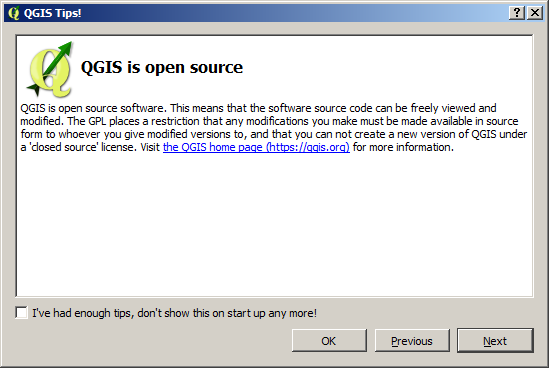
3. When you first open QGIS, you will see the QGIS Tips! Window, click OK to close it.

Figure 0.9: Screenshot of QGIS welcome screen

1.2.2 Change QGIS Language (optional)

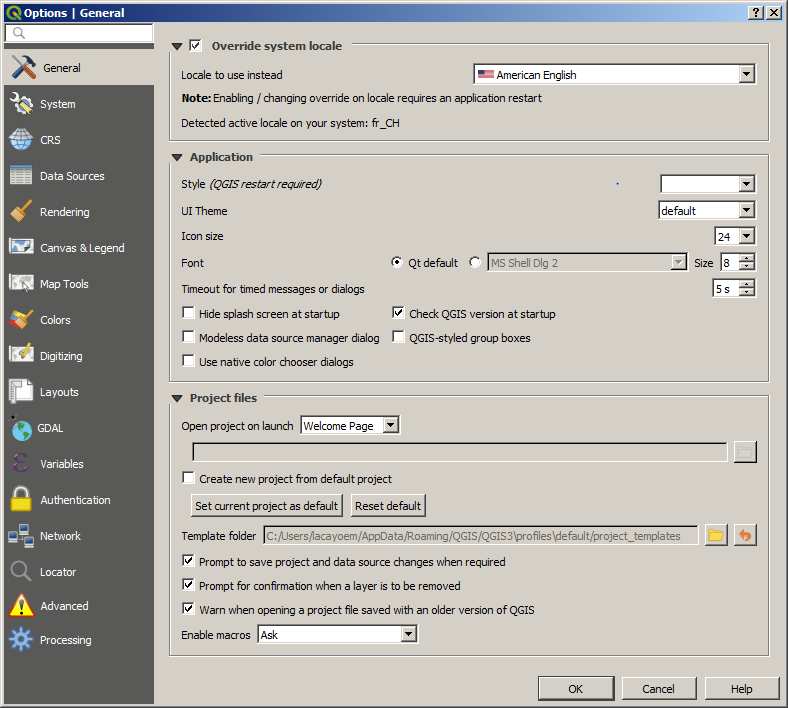
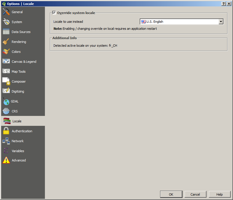
1. Use Settings > Options to change the language. Under General check the box next to Override system locale and change Locale to use instead to your preferred language. Click OK to save the change and restart QGIS to view it in the new language.

   

   Figure 0.10: Screenshot of QGIS general settings for language override

1.2.3 Area of Interest

The area of interest (AOI) is the place of your analysis and having it in the ESRI Shapefile format can be useful during preprocessing to reduce the data to only that which you will actually use. There are several ways to get an area of interest polygon for your analysis. If your analysis area is an official administrative unit it may be possible to obtain a Shapefile directly from the authorities responsible for this area. In other cases, you may have to create the Shapefile yourself using the coordinates for the area. For hydrological analysis it is ideal if the area of interest corresponds to watersheds or subwatersheds since these are the units at which a hydrologic process typically occurs.

Note: Consider creating an initial area of interest with the following instructions, which you can then use to help select the final area of interest based on the watersheds as detailed in the section Watersheds.

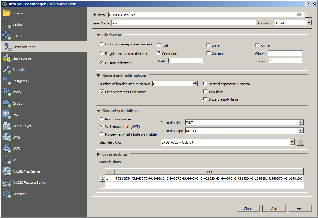
1. Create a text file with the polygon defined in the WKT format. See the example file aoi.txt. The coordinates are a closed list, meaning the first and last point are the same. It is conventional to list the points in clockwise order.

2. Use Layer > Add Layer > Add Delimited Text Layer to create a layer from aoi.txt. Click Add and then Close.

Note: If you are using latitude and longitude the correct projection is typically EPSG:4326.

Figure 0.11: Screenshot of QGIS delimited text data source manager dialog box for area of interest

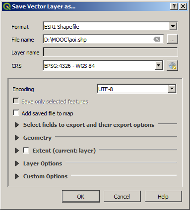
3. The area of interest is now listed in the Layers panel. Right click it and use Export > Save Features As to save it to the ESRI Shapefile format with the options below.

Figure 0.12: Screenshot of QGIS layers panel save vector layer dialog box for area of interest Shapefile

Note: See Projections in the appendix for more information.

1.2.4 Precipitation

The precipitation comes from WorldClim dataset.

1. Use Layer > Add Layer > Add Vector Layer to add all 12 precipitation rasters to QGIS.

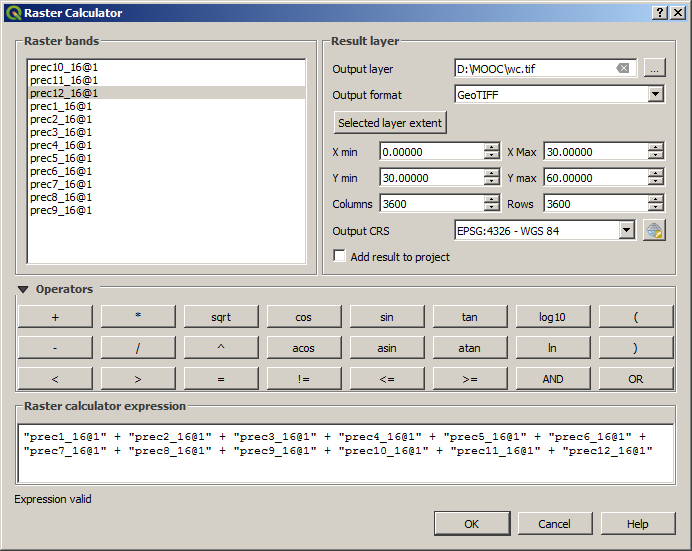
2. Use Raster > Raster Calculator to create wc.tif by adding together all 12 precipitation rasters using the + operator.

Figure 0.13: Screenshot of QGIS raster calculator dialog box for annual precipitation

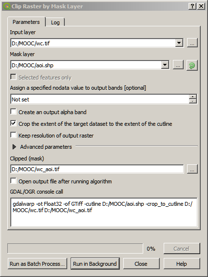
3. Use Raster > Extraction > Clip Raster by Mask Layer to create wc_aoi.tif by clipping wc.tif with aoi.shp.

Figure 0.14: Screenshot of QGIS clip raster by mask layer dialog box for area of interest annual precipitation

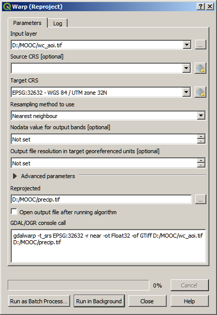
4. Use Raster > Projections > Warp (Reproject) to create precip.tif by projecting wc_aoi.tif to the analysis projection EPSG:32632.

Figure 0.15: Screenshot of QGIS warp raster dialog box for reprojected area of interest annual precipitation

1.2.5 Average Annual Reference Evapotranspiration

The average annual reference evapotranspiration comes from the CGIAR CSI dataset.

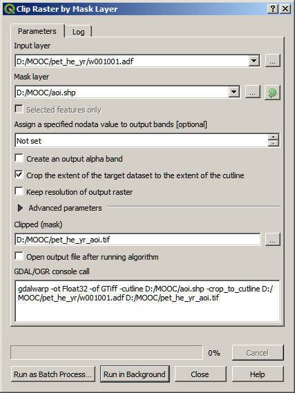
1. Use Raster > Extraction > Clip Raster by Mask Layer to create pet_he_yr_aoi.tif by clipping pet_he_yr/w001001.adf with aoi.shp.

Figure 0.16: Screenshot of QGIS clip raster by mask layer dialog box for area of interest average annual reference evapotranspiration

2. Use Raster > Projections > Warp (Reproject) to create eto.tif by projecting pet_he_yr_aoi.tif.

Figure 0.17: Screenshot of QGIS warp raster dialog box for reprojected area of interest average annual evapotranspiration

1.2.6 Plant Available Water Content and Root Restricting Layer Depth

The plant available water content and root restricting layer depth come from the Harmonized World Soil Database.

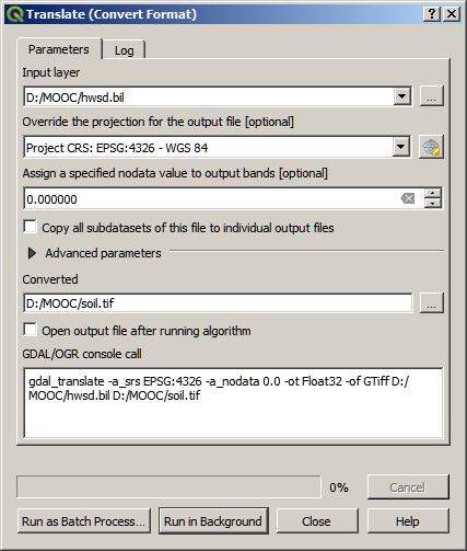
1. Use Raster > Conversion > Translate to create soil.tif by converting hwsd.bil with the options below. QGIS may not recognize the projection so it is important to specify EPSG:4326 in the Override the projection for the output file parameter.

Figure 0.18: Screenshot of QGIS raster format conversion dialog box for plant available water content and root restricting layer depth

2. Use Raster > Extraction > Clip Raster by Mask Layer to create soil_aoi.tif by clipping soil.tif with aoi.shp. Be sure to specify the Output data type as Byte.

Figure 0.19: Screenshot of QGIS clip raster by mask layer dialog box for area of interest plant available water content and root restricting layer depth

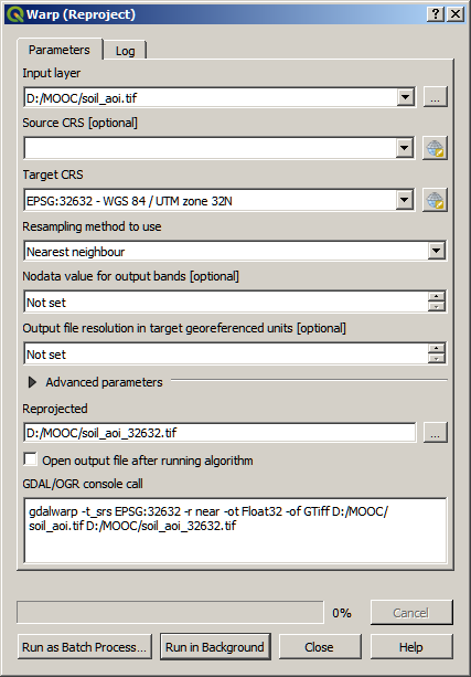
3. Use Raster > Projections > Warp (Reproject) to create soil_aoi_32632.tif by projecting soil_aoi.tif to the analysis projection EPSG:32632.

Figure 0.20: Screenshot of QGIS warp raster dialog box for reprojected area of interest plant available water content and root restricting layer depth

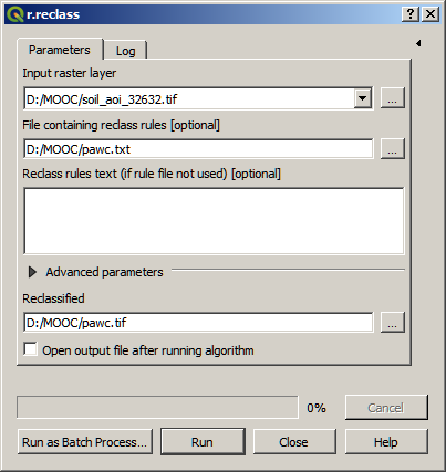
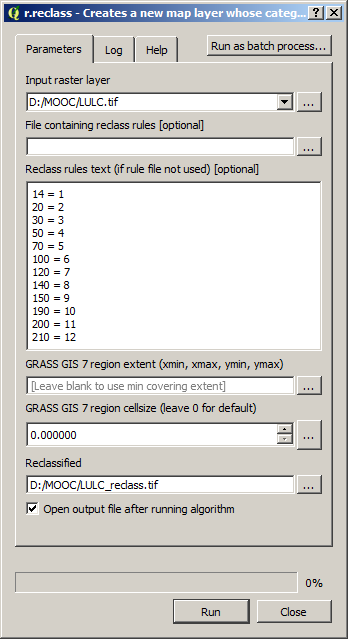
4. Use Processing > Toolbox > GRASS > Raster > Raster (r.*) > r.reclass to create pawc.tif by reclassify soil_aoi_32632.tif with the provided reclass rules pawc.txt.

Figure 0.21: Screenshot of QGIS raster reclass dialog box for reprojected area of interest plant available water content

Note: The reclass rules in pawc.txt and roots.txt are global and come from the metadata for the Harmonized World Soil Database. This allows the conversion of the soil mapping unit (MU_GLOBAL) values in hwsd.bil to corresponding characteristics. In pawc.txt the available water content (AWC_CLASS) is divided by the reference soil depth (REF_DEPTH) for the plant available water content fraction. In roots.txt the range values for the obstacles to roots depth (ROOTS) categories are averaged and converted to millimeters for the depth to root resistance.

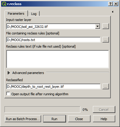
5. Use Processing > Toolbox > GRASS > Raster > Raster (r.*) > r.reclass to create depth_to_root_rest_layer.tif by reclassify soil_aoi_32632.tif with the provided reclass rules roots.txt.

Figure 0.22: Screenshot of QGIS raster reclass dialog box for reprojected area of interest root restricting layer depth

1.2.7 Land Use Land Cover

The land use land cover comes from the GlobCover dataset.

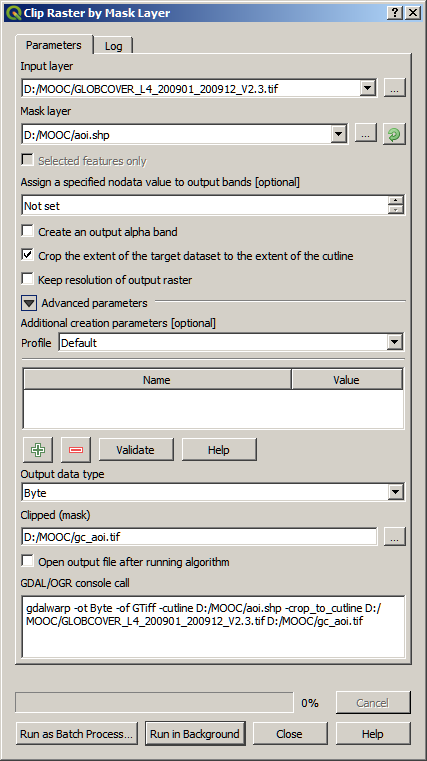
2. Use Raster > Extraction > Clip Raster by Mask Layer to create gc_aoi.shp by clipping the GLOBCOVER_L4_200901_200912_V2.3.tif with aoi.shp.

Figure 0.23: Screenshot of QGIS clip raster by mask layer dialog box for area of interest landuse and land cover

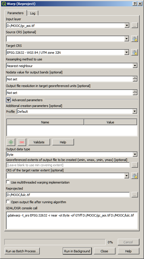
3. Use Raster > Projections > Warp (Reproject) to create lulc.tif by projecting globcover_aoi.tif to the analysis projection of EPSG:32632.

Figure 0.24: Screenshot of QGIS warp raster dialog box for reprojected area of interest landuse and land cover

1.2.8 Watersheds

The watersheds come from the HyrdoBASIN dataset.

1. Use Layer > Add Layer > Add Vector Layer to add aoi.shp and the watershed layer.

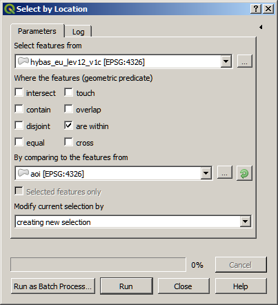
2. Use Vector > Research Tools > Select by Location to select the watersheds that are within the area of interest.

Note: Depending on the extent of the analysis you may wish to set Where the features (geometric predicate) to another value, but be aware that if and where the watersheds go beyond the boundaries of the other clipped and projected datasets some results will be incorrect.

Figure 0.25: Screenshot of QGIS select by location dialog box for area of interest watersheds

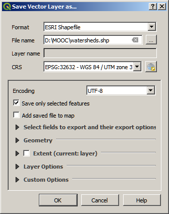
3. Right click on the watershed layer and use Export > Save Features As to save the selected features to the analysis projection of EPSG:32632.

Figure 0.26: Screenshot of QGIS layers panel save vector layer dialog box for area of interest watersheds

4. Use Layer > Add Layer > Add Vector Layer to add the new watersheds.shp with the selected watersheds.

5. Right click on the watersheds.shp layer and select Open Attribute Table.

6. Use the Open field calculator abacus icon to open the Field Calculator.

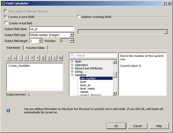
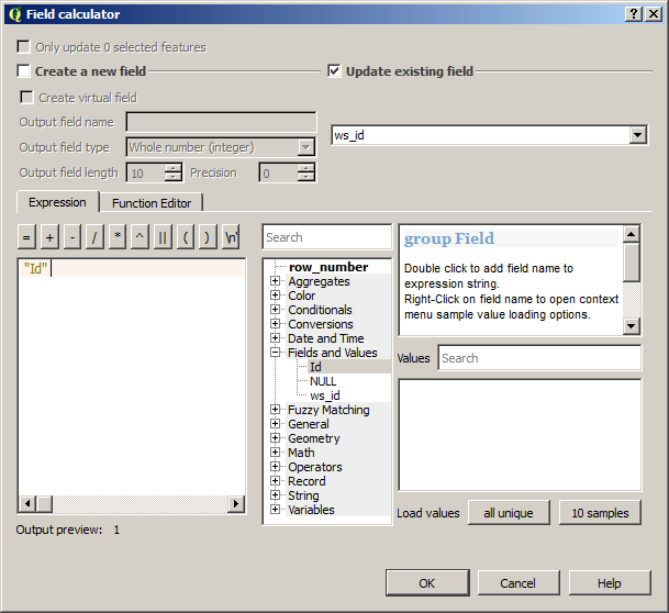
7. Use the Field Calculator to create a new field named ws_id with the value @row_number.

Note: The Output field length is the maximum number of digits that can appear in the field. For example, if you had 10 watersheds you need a field length of 2 because there are 2 digits in the number 10.

Figure 0.27: Screenshot of QGIS field calculator dialog box for watershed identifiers

8. Now the attribute table should show a new column named ws_id with row numbers in it. Click on the Toggle editing mode pencil icon to stop editing and save edits.

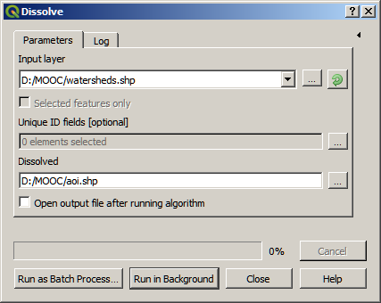
9. Use Vector > Geoprocessing Tools > Dissolve to create an updated aoi.shp from watersheds.shp.

Figure 0.28: Screenshot of QGIS dissolve vector layer dialog box for watersheds area

1.2.9 Biophysical Table

The biophysical table can be created in a variety of ways, but it can be useful to first generate a template from the count of the pixel values.

1. Use Processing > Toolbox > GRASS > Raster (r.*) > r.stats to create the HTML report counts.html with the exact options as below. Be sure to specify lulc.tif in the Name of input raster map parameter.

Figure 0.29: Screenshot of QGIS raster statistics dialog box for reprojected area of interest landuse and land cover pixel counts

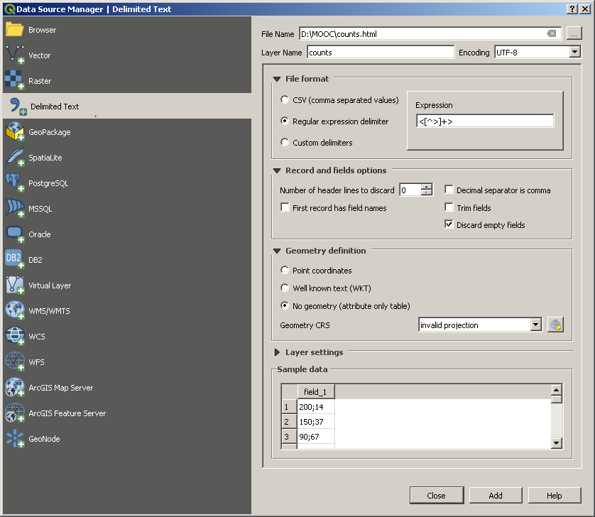
2. Use Layer > Add Layer > Add Delimited Text Layer to create a table by removing the HTML formatting by specifying the Regular expression delimiter as <[^>]+>

Figure 0.30: Screenshot of QGIS delimited text data source dialog box for reprojected area of interest landuse and land cover pixel count table

3. Right click on the table and use Export > Save Features As to create counts.csv with the current formatting.

Figure 0.31: Screenshot of QGIS save vector layer dialog box for comma separated values of reprojected area of interest landuse and land cover pixel count table

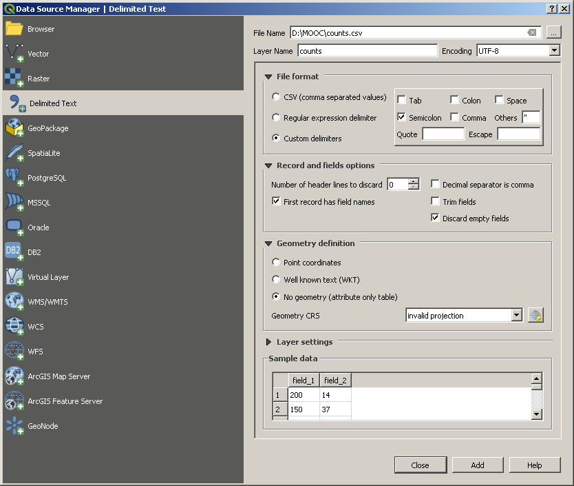
4. Use Layer > Add Layer > Add Delimited Text Layer to remove the last undesired formatting elements from counts.csv.

Figure 0.32: Screenshot of QGIS delimited text data source manager dialog box for comma separated values of reprojected area of interest landuse and land cover pixel count table

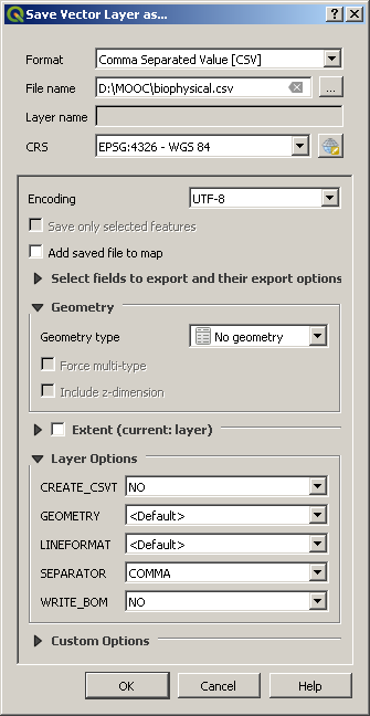
5. Right click on the table and use Export > Save Features As to create biophsyical.csv with the current formatting.

Figure 0.33: Screenshot of QGIS save vector layer dialog box for comma separated values of reprojected area of interest landuse and land cover pixel count table

Use biophysical.csv as a template and fill in the correct data with the methods highlighted in Appendix 1.

1.2.10 Z parameter

See Appendix 1 for more information about the Z parameter.

1.2.11 Reclass Rules for Rasters

In this document we use Processing > Toolbox > GRASS > Raster > Raster (r.*) > r.reclass to reclass rasters.

Note: complete documentation on the reclass function can be found at https://grass.osgeo.org/grass74/manuals/r.reclass.html

The reclass rules text uses the following format, which can either be specified in a text file or manually using the following format:

10 = 1

12 13 = 2

14 thru 20 = 3

* = NULL

Figure 0.34: Screenshot of QGIS raster reclass dialog box with inline reclass rules

1.2.12 Adding Fields to a Shapefile

1. Use Layer > Add Layer > Add Vector Layer to open the shapefile that you want to which you want to add a field.

2. Right click and select Open Attribute Table.

3. Click on the Toggle editing mode pencil icon to enable editing.

4. Click on the New field table icon to add a new field.

5. Manually enter the values for the new field or use the calculator to calculate them.

Note: The Open field calculator abacus icon can create new fields directly.

Figure 0.35: Screenshot of QGIS field calculator dialog box

1.2.13 Projections

Geography is literally the study of Earth and a projection, or coordinate system, describes how to divide the Earth into pieces so that places can be located. Coordinate systems include a formal description of the shape of Earth, the area where the coordinate system can be used, and the unit of measure. The unit of measure is either angular or linear. Angular units are those like degrees that measure parts of a rotation. Linear units are those like meters that measure distances.

There are thousands of commonly used coordinate systems each with their own advantages. All coordinates have a coordinate system that must be specified. Projecting data means to change the coordinate system, although it should be noted that informally “projected data” is sometimes used to refer to data with a coordinate system that uses linear units.

For convenience, QGIS will display together data with different coordinate systems. However, different datasets must be in the same coordinate system when they interact as is the case when clipping. For this reason, it is useful to know how to identify the coordinate system of data and project data into another coordinate system.

1. Start by first adding the shapefile for your analysis area to QGIS. See Create Area of Interest above for details. After you add your shapefile to QGIS you will see it listed in the Layers panel on the left.

Note: If you cannot see the layers panel you can enable it by selecting View > Panels > Layers.

2. Right click on your layer and select Properties. Under the Information tab you will see a section named Information from provider with an entry CRS, which is an abbreviation for Coordinate Reference System, and where the coordinate system is identified. In the example analysis area you will see EPSG:4326 - WGS 84 – Geographic. Close the information before continuing to the next step.

3. Use Vector > Data Management Tools > Reproject Layer to project your data to the corresponding UTM zone. For the example analysis area set the Target CRS to EPSG:4326 as this is the corresponding UTM zone.

Note: ESPG:4326 is a global projection, which we use in this document for the initial steps of processing global layers. However, the example analysis area falls within EPSG:32632, one of 60 UTM zones defined for specific locations on Earth, and it is EPSG:32632 that will be used for analysis. The correct UTM zone for your chosen analysis area may be different. For detailed information about specific projections see http://spatialreference.org/

1.3 Running InVEST

1.4 Visualizing Results in QGIS

1. Download the latest version of QGIS from http://qgis.org/ and install it. This tutorial was made for QGIS 2.16.1 Nodebo.

2. Run QGIS

3. When you first open QGIS, you will see the QGIS Tips! Window, click OK to close it.

Figure 0.36: Screenshot of QGIS welcome screen

4. If desired you can change the language of QGIS by selecting Options from the Settings menu. Under Locale check the box next to Override system locale and change Locale to use instead to your preferred language. Click OK to save the change and restart QGIS to view it in the new language.

Figure 0.37: Screenshot of QGIS general settings for language override

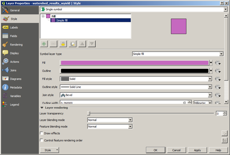
5. Select Layer > Add Layer > Add Vector Layer and browse to the output from the InVEST Water Yield model and select watershed_results_wyield.shp. The watersheds will appear in a random color. In the Layers Panel right click on the layer and select properties. Under the Style tab there is the symbology hierarchy with Fill > Simple fill. Select Simple fill in the symbology hierarchy and under Symbol layer type you will see the symbology definition. Next to the current fill color click on the down arrow and select Transparent fill from about the color wheel. Next change the Outline width to 0.5 mm.

Figure 0.38 Screenshot of QGIS vector layer properties dialog box for single symbol style

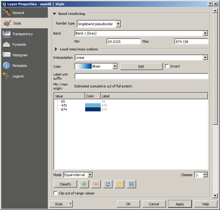
6. Select Layer > Add Layer > Add Raster Layer and browse to the output from the InVEST Water Yield model and select wyield.tif. The water yield will appear in grayscale colors. In the Layers Panel right click on the layer and select properties. Under the Style tab you will see Render type. Change Render type from Singleband gray to Singleband pseudocolor and change Color to Blues, Mode to Equal interval, and Classes to 3.

Figure 0.39: Screenshot of QGIS raster layer properties dialog box for singleband pseudocolor band rendering

7. Right click wyield.tif in the Layers Panel and select Zoom to Layer this will make it easy to set the extent in the Print Composer.

8. Open QGIS and select New Print Composer from the file menu.

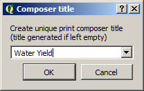
9. Enter Water Yield as the title in the Composer title window and click OK.

Figure 0.40: Screenshot of QGIS print composer dialog box for map layout management

10. Set the desired page properties Composer > Page Setup in this tutorial we will use A4 paper.

11. Select View > Show Grid and View > Snap to Grid

12. Select Layout > Add Map use the cross hairs to draw a map area. Click on the Item properties tab on the right sided. Under Position and size set X to 10 mm, Y to 10 mm, Width to 277 mm, Height to 190 mm. Under Extents click on Set to map canvas extent. Under Main properties change Scale to a round number that still accommodates the map.

13. Rename the layers in the Layers Panel by right click on each layer and selecting Rename.

14. Select Layout > Add Legend and use the cross hairs to draw in a legend in the lower right corner. Click on the Item properties tab on the right sided. Under Position and size change the Width to 35 mm, Height to 45 mm, Reference point to the lower right corner, X to 287 mm, and Y to 150 mm.

15. Select Layout > Add Label use the cross hairs to draw at the top. Click on the Item properties tab on the right sided. Under Main properties enter Water yield in the Tana River Basin. Under Appearance change the Horizontal alignment to Center and change Vertical alignment to Middle. Under Font change the Size to 24. Under Position and size set X to 10 mm, Y to 10 mm, Width to 277 mm, Height to 20 mm.

16. Select Layout > Add Label use the cross hairs to draw in the lower left corner. Click on the Item properties tab on the right sided. Under Main properties enter Data Source: Natural Capital Project. Under Appearance leave the Horizontal alignment at Left and change Vertical alignment to Bottom. Under Font change the Size to 12. Under Position and size set X to 10 mm, Y to 200 mm, Width to 75 mm, Height to 10 mm, and Reference point to the lower left corner.

17. Select Layout > Add Label use the cross hairs to draw in the lower left corner. Click on the Item properties tab on the right sided. Under Main properties enter Created by [Your Name]. Under Appearance leave the Horizontal alignment at Right and change Vertical alignment to Bottom. Under Font change the Size to 12. Under Position and size set X to 287 mm, Y to 200 mm, Width to 75 mm, Height to 10 mm, and Reference point to the lower right corner.

18. Select Layout > Add Scalebar use the cross hairs to draw in the bottom right. Click on the Item properties tab on the right sided. Under Segments change Segments to left 0 and right 6, select Fixed width and set the value to 5000 units. Under Position and size set X to 148.5 mm, Y to 200 mm, Width to 100 mm, Height to 20 mm, and Reference point to the middle center corner.

19. Select Layout > Add Image use the cross hairs to draw in the lower left corner. Click on the Item properties tab on the right sided. Under Search directories select the desired north arrow image from the provided ones. Under Position and size set X to 210 mm, Y to 150 mm, Width to 15 mm, Height to 25 mm, and leave the Reference point to as the top left.

20. Now that you know how to make a basic map for water yield try making maps of the other outputs from InVEST.

Figure 0.41: Map of example InVEST water yield model